Backpropogation in batch normalization...
Neural networks are considered powerful because of their ability to adapt and improve over time. But how does a neural network exactly improve itself, you ask? The secret sauce is known as backpropogation. Now this may sound fancy, but backpropogation is nothing more than calculation of subgradients which when added to (or subtracted from) the respective input would ideally lead to maximize (or minimize) the cost function. In the following post, I’ll refer coursework from the amazing lecture series of CS231n provided by the good folks over at Stanford University. If you haven’t already, head over here to access the course in its entirety.
What is Batch Normalization (and why do we need it)?
If we were to look at the wiki, Batch Normalization…
“…can mitigate the problem of internal covariate shift, where parameter initialization and changes in the distribution of the inputs of each layer affect the learning rate of the network.”
One might notice the term internal covariate shift. Internal covariate shift is a phenomenon that occurs when the input to the network is very different from the inputs the network has been trained on so far. This causes the training procedure (and consequently the convergence) to slow down, as the hidden layers try to adapt to the new distribution. Experiments have shown that this phenomenon can occur in between subnetworks and layers as well. Previous techniques like normalizing activations are known to help alleviate covariate shift in the overall network. So how do we generalize this to remove internal covariate shift from within a network? By normalizing the batches of images that are fed into a layer!

Before getting into the details, there’s a great explanation by Frederik Kratzert over here which this post is heavily inspired from. With that out of the way, let’s look at how Batch Normalization functions (and how it is actually implemented)
Forward pass
Implementing the forward pass for Batchnorm is fairly starightforward. Let’s take a look at the implementation from the paper by Ioffe and Szegedy.
As the name suggests, we calculate the batch statistics (the batch mean and variance) and normalize the input using those statistics. One might notice that the result is then scaled and shifted by gamma and beta parameters. These are learnable parameters that enable the input to regain their original distibution (given certain conditions are satisified), or any other distribution for that matter of fact. But since these are learnable, we leave it up to the network to decide what’s best for a particular case.
Backward pass
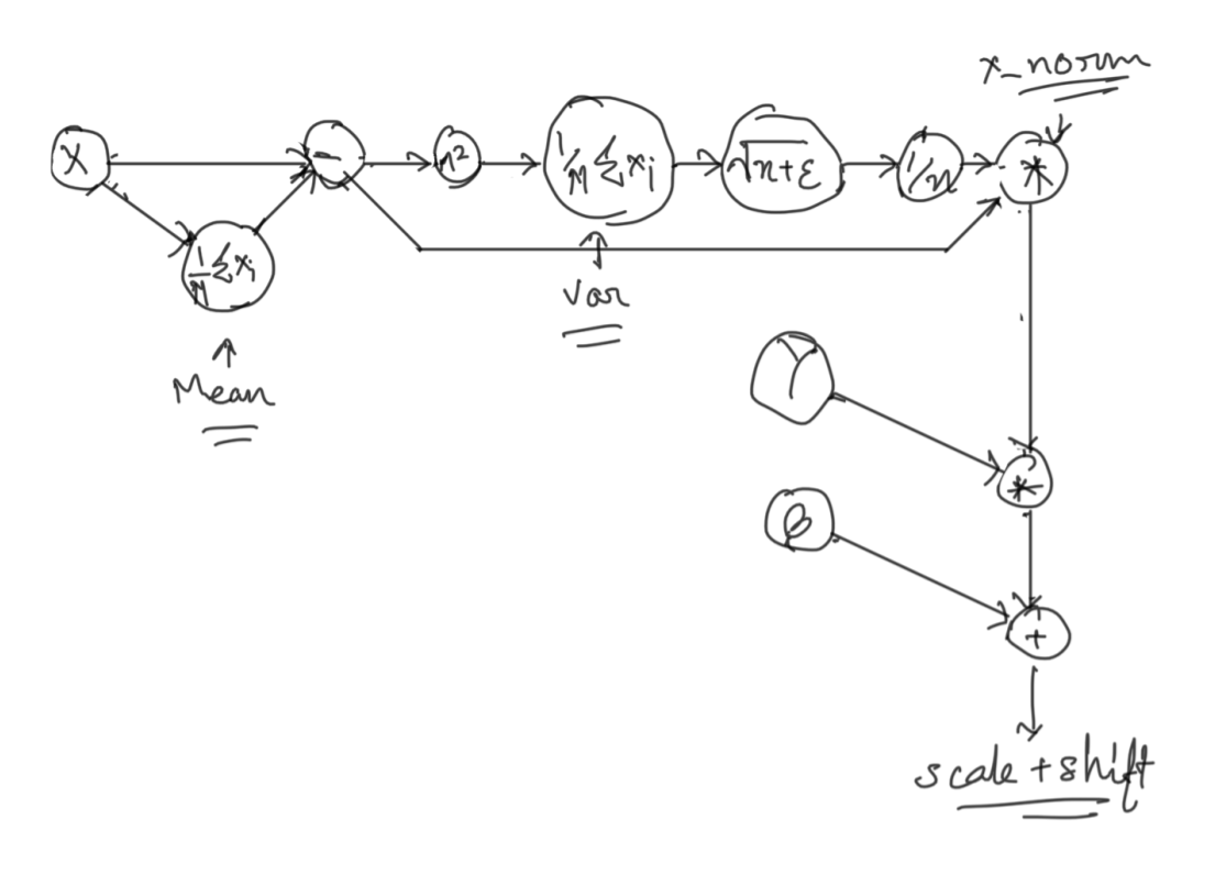
This is where things started getting a bit hairy (for me atleast). It’s easy to numerically calculate the gradient, but for us to understand the actual flow of the gradient back to the input, it’s very important to understand computational graphs. Before we can dive into the graph for the backward flow, lets take a look at the computational graph for the forward pass.

This is the same representation of the formula given in the Fig 2. We just broke down the operations into differentiable pieces to simplify the understanding.
We backprop through this graph one node at a time. We shall use the power of chain rule of differentiation to calculate gradient at each step. Let’s begin at the final node:
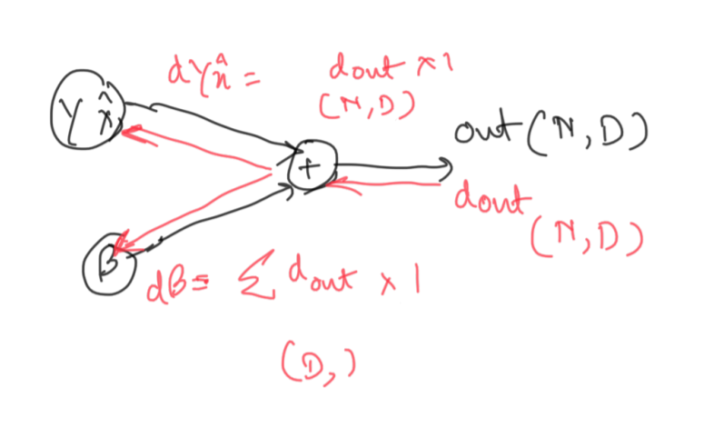
Notice how the node performs an addition operation. In case of addition, the subgradient is 1 w.r.t. both the inputs. So we multiply the gradient of the final loss with 1 at both splits. We also need to take care that the dimentsionality of the features are maintained, which is why we sum over N to calculate the subgradient w.r.t. beta.
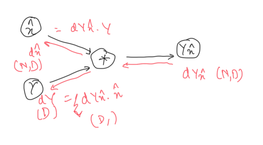
Unlike addition, multiplication divides the inputs s.t. the other input stays as a constant. Thus, subgradients are calculated as multiplication of the other input with the previous subgrad.
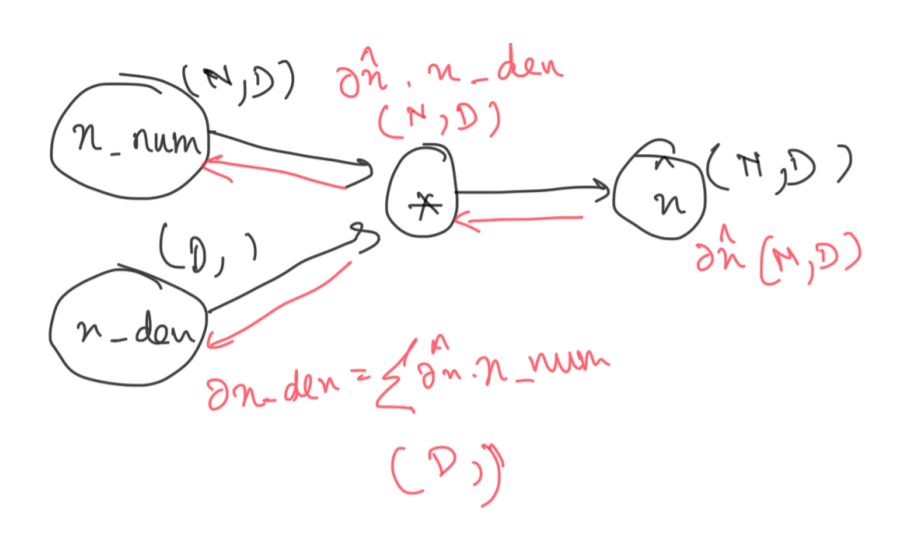
We follow the same steps as before, since the operation is multiplication.
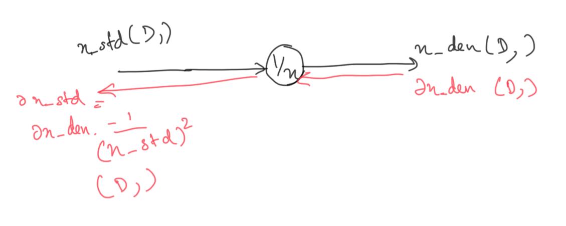
The derivative of \(1/x\) is \(-1/x^2\), which is then multiplied with the input from the last backward pass.
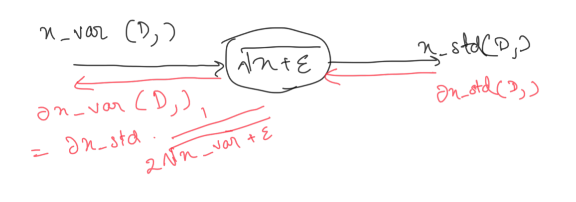
Just like before, we calculate the local gradient.
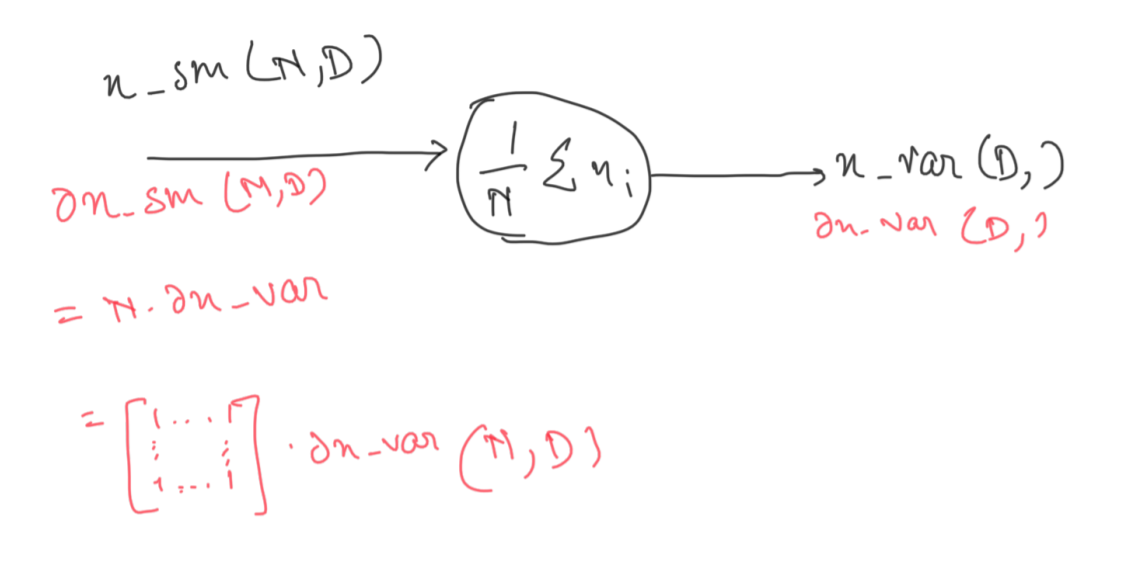
This step might look tricky, but it really isn’t. We need to make sure that the dimensions are preserved w.r.t the inputs. Now since we have a (D,) dimension vector coming in from the previous backward pass that needs to be transformed into an (N, D) matrix, the local gradient would an (N, D) matrix of 1’s to transform the vector into the required shape.
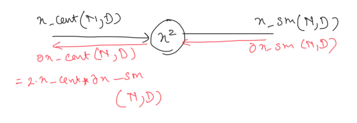
Not much to explain.
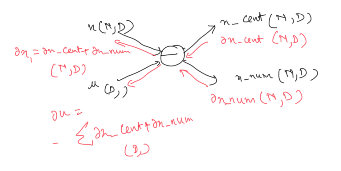
This might seem confusing, but we can just apply a combination of what we have learnt till now to calculate gradient at this node. For the incoming subgradients at the node, we simply sum them up. During the backprop, the operation is nothing but an addition of a positive and a negative number which we have already performed above.
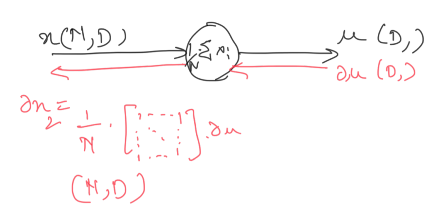
Again, an operation similar to the one we performed before.
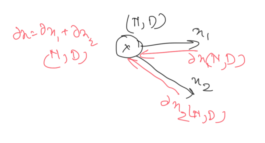
Just like the example before the previous one, we sum the incoming subgradients to get the final value for the input. This is the final gradient dx that we set out to compute.
And that’s all there is to it! Laying out the computational graph is more of a tedious task than a difficult one. And with modern machine learning libraries doing the work for us, it’s more about the understanding of the concepts than the final implementation. I hope this helps out people as much as it did for me. Until next time!
Enjoy Reading This Article?
Here are some more articles you might like to read next: